Bring Your Own Model (BYOM)

This section focuses on one of the key customization opportunities offered by Vitis AI.

The Bring Your Own Model (BYOM) allows you to use your own pretrained model (PyTorch, TensorFlow, ONNX, etc.) for AI inference on AMD hardware platforms, leveraging the NPU IP, tools, and libraries provided by Vitis AI.

The typical workflow for executing inference with NPU IP begins with training the network. However, the NPU IP is not involved in model training because it is not a training accelerator, but rather an inference accelerator.

The following figure describes the workflow for executing inference with NPU IP.

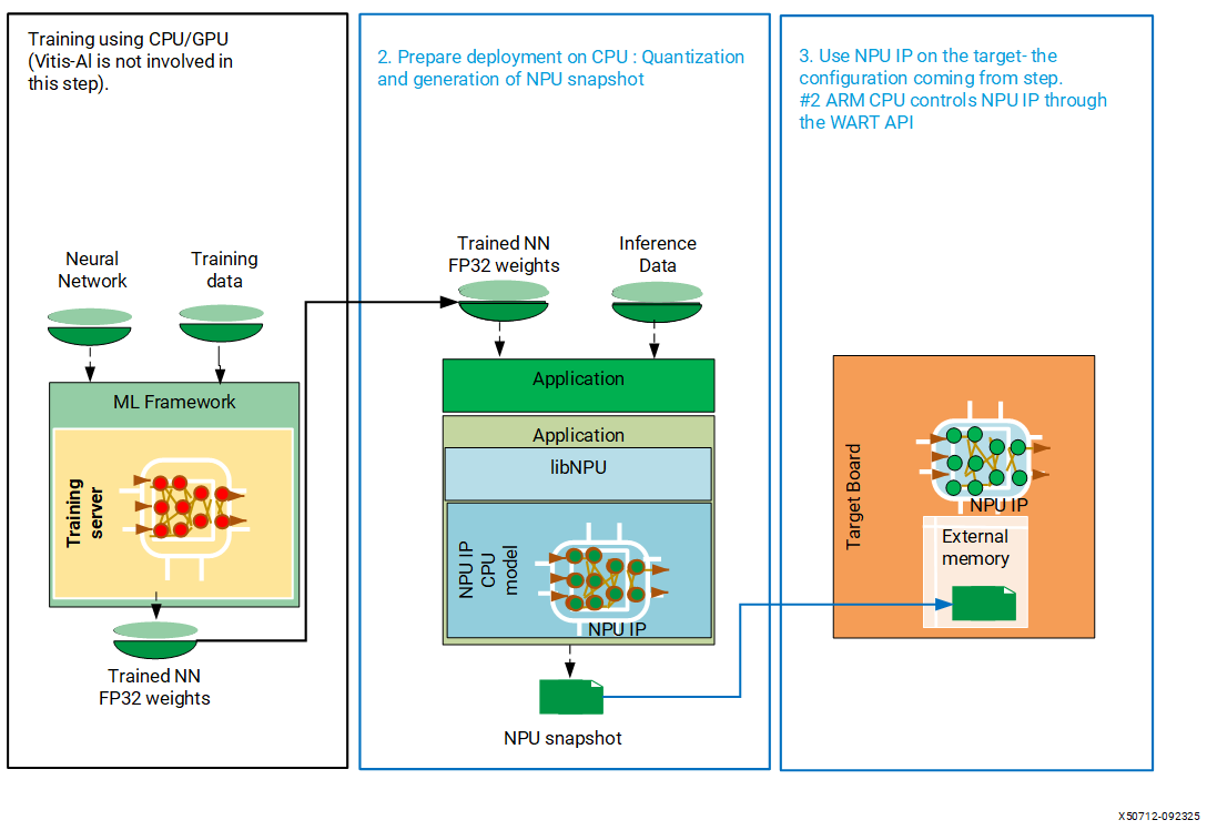
The first step in the previous diagram is “Model Training,” in which Vitis AI (NPU IP) is not involved. The second step is the model compilation process, in which the software stack of the NPU IP generates a description of the configuration of the NPU IP for the trained model, tailored for inference on NPU IP hardware. This description is commonly referred to as a snapshot. A snapshot contains all the necessary information required for efficient execution, including layer descriptions, weights, and input/output shapes.

The BYOM workflow addresses the following steps:

• Generating Snapshot For Your Model: The procedure includes graph management, model quantization, and compilation of your custom model.

• Deploying Your Model on Target Board: The operation includes deployment of custom model on the embedded platform (target hardware), and AI inference of the user generated snapshot(s).

1. Generating Snapshot For Your Model

The snapshot generation process performs the following tasks, and the Vitis AI NPU software stack takes care of all these stages automatically.

• Graph Management

• Quantization

• Compilation

Graph Management

Graph management is the first stage of the snapshot generation process, and it performs the following sub-tasks.

• Converts your model to ONNX,

• Graph splitting, and

• Graph optimization

Note

Your model is expected to be ONNX compliant. If it is not ONNX compliant, then Vitis AI software cannot compile the model and results in a compilation error.

The Vitis AI NPU software stack converts your model to ONNX and then splits the main model graph into sub-graphs named CPU sub-graph and Vitis AI Software (FPGA) sub-graph, depending on the layers supported by NPU IP. The CPU sub-graphs are run by the ONNX runtime, and the Vitis AI software sub-graph is accelerated by the NPU IP. The following is an example of graph splitting visualized using Netron.

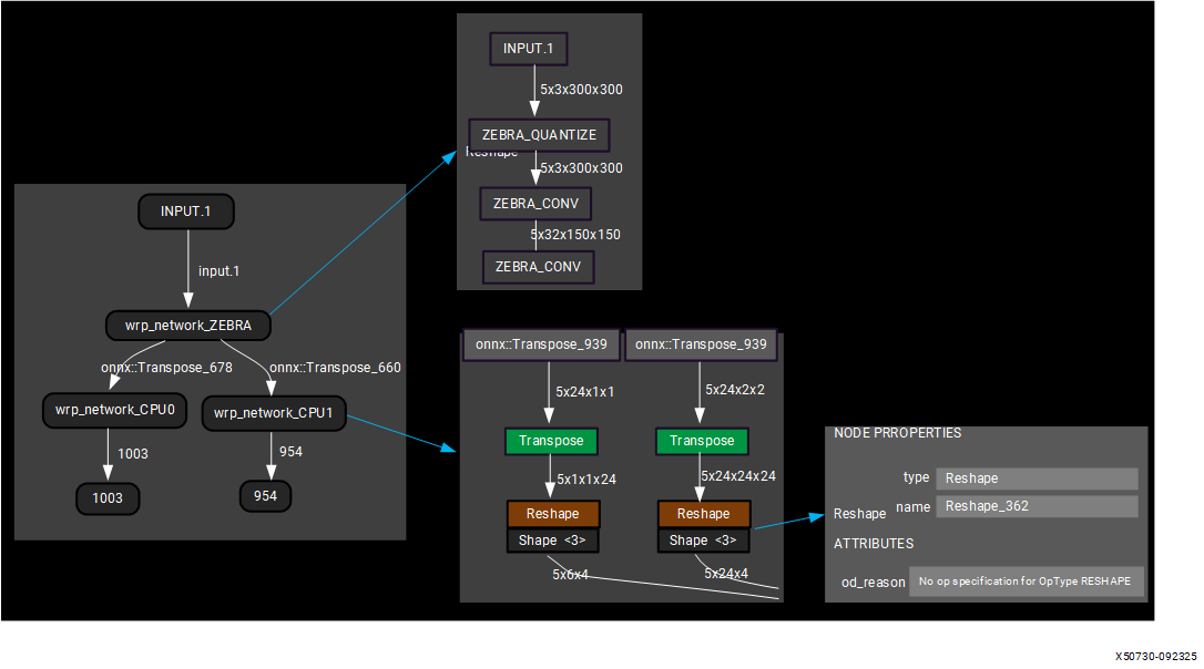
It is important to note that sub-graphs are only generated after the compilation stage. You can use a visualization tool such as Netron to analyze the layers within the neural network model. These sub-graphs are simplified using a set of tools, including ‘pattern matching search and replace,’ provided by the Vitis AI NPU software stack. The goal is to ensure that as many operators as possible can run on the device. For example, the ‘Convolution (Conv_3),’ ‘Batch Normalization (BatchNormalization_4),’ and ‘Activation (Relu_5)’ layers are combined into a single ‘Convolution (Conv_3)’ layer.

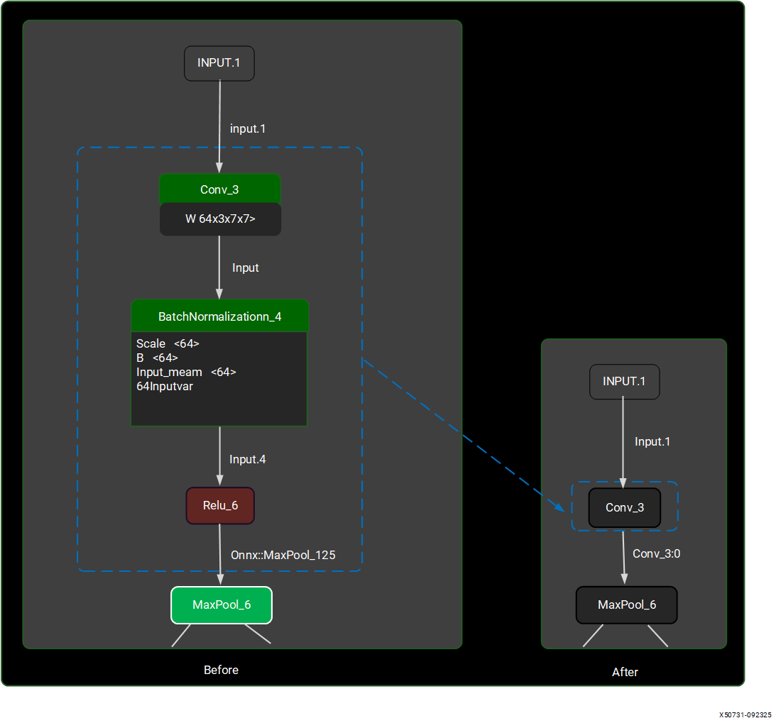
After the graph optimization is done on sub-graphs, the optimized/simplified graph is used for quantization, which is explained in the following section.

Quantization

The Vitis AI tool offers an auto quantization feature, meaning that quantization is automatically enabled while compiling the model.

Deploying neural networks on AMD NPUs becomes more efficient through the use of integer quantization, which reduces energy consumption, memory footprint, and the bandwidth required for inference.

AMD’s general-purpose NPUs support INT8 (8-bit integer) quantization for trained networks. For many real-world datasets, the range of weights and activations at a particular layer is often much narrower than what can be represented by a 32-bit floating-point number. By applying a scaling factor, it is possible to represent these weights and activations with integer values. The impact of INT8 quantization on prediction accuracy is typically minimal, often less than 1%. This level of precision is maintained across various applications, including those that process image and video data, point-cloud data, and sampled-data systems such as specific audio and RF applications.

This section explains the quantization/compilation process, along with suggestions for fine-tuning the accuracy. Before proceeding with quantization/compilation using Vitis AI, ensure that you meet the necessary prerequisites.

Prerequisites

You need the following prerequisites to generate a snapshot for your custom model:

• Docker: Ensure that Docker is running. Refer to the Install And Verify Docker section in Software Installations to launch Docker.

• Custom model: The model (for which the snapshot is generated) is located in the MY_APP directory on the host machine.

  Note

  You create an MY_APP folder on the host machine and copy the custom model and dataset into that folder.

• Dataset: A valid dataset (for the custom model) resides in the MY_APP directory on the host machine.

• Python application: A Python application runs the neural network using supported frameworks like PyTorch, ONNX Runtime, or TensorFlow. It performs inference on a valid input dataset, on the CPU or GPU of an x86 host. The Python application, named my_network_inference.py, is used as an example in the MY_APP directory. It contains this simple example code snippet that uses ResNet50 from torchvision. For simplicity, proper pre-processing and top1 or top5 codes are omitted. However, the next Python code is sufficient for the NPU software stack to perform the quantization and compilation of the ResNet50 model. The Python code includes nothing specific to the NPU software stack. It is a valid Python program that you can execute with default Python packages.

import torchvision
import torch

transform = torchvision.transforms.Compose([torchvision.transforms.ToTensor()])

# Replace PYTORCH_IMAGENET with the actual path where you have saved the ImageNet dataset
imgnet_data = torchvision.datasets.ImageNet("PYTORCH_IMAGENET", split='val', transform=transform)
data_loader = torch.utils.data.DataLoader(imgnet_data, batch_size=1, shuffle=False)

model = torch.hub.load('pytorch/vision:v0.10.0', 'resnet50', pretrained=True)

for i, (in_data, y) in enumerate(data_loader):
    preprocess = in_data
    # pseudocode, replace with your pre-processing routines

    out = model(preprocess)
    # run inference model
    print("Process ", i)

    if i > 100:
        break

Note

You might use your custom model, dataset, and an application (that runs the custom model on the host machine) and attempt the following steps.

For illustration purposes, assume you have a Python script named my_network_inference.py that contains the above Python code, which runs the inference of your floating-point model (for example, a ResNet50 model). This script includes the correct pre-processing and post-processing routines and points to the original floating-point model of the neural network, along with the test dataset used during its original training to achieve the best average prediction accuracy.

When you execute the script my_network_inference.py on your host machine, it runs the network on many inputs and eventually outputs an accuracy metric. You can refer to the following section for fine-tuning the accuracy.

Measure Accuracy

First, collect the best achievable accuracy by running the network on the CPU, then running the network on the emulated NPU (on the CPU) with the default parameters to establish a baseline.

Execute the following commands within the Docker container.

# Go to Vitis AI source code
$ cd <path_to_Vitis_AI_folder>

# Launch Docker
$ ./docker/run.bsh -v <path_to_MY_APP>:/MY_APP

# Go to MY_APP folder within Docker. The MY_APP folder contains your custom model, Python application for inference, and required dataset, etc.
$ cd /MY_APP

# Run on CPU to get reference FP32 accuracy
$ python3 my_network_inference.py

# Activate NPU (set the Vitis AI environment)
$ source $VITIS_AI_REPO/npu_ip/settings.sh

# Run on NPU
$ python3 my_network_inference.py

After executing the previous commands, you obtain the inference and accuracy results on both CPU and NPU.

Quantization Options

The Vitis AI tool provides various quantization options and the following environment variables can be used to change the default options of the quantization process of the NPU IP. Changing the QUANTIZATION or DEEPQUANTIZATION options might result in better quality depending on the neural network.

Variable environment	Description
VAISW_RUNSESSION_DIRECTORY=path	Directory where the model configuration is saved. Default: ~/.amd/vaisw
VAISW_SNAPSHOT_DIRECTORY=path	Set the path of the snapshot directory. Default: <runSessionDirectory>/snapshot
VAISW_QUANTIZATION_NBIMAGES=4	Control the number of images for quantization tuning. Default: 4
VAISW_QUANTIZATION_MODE=dynamic	Choose another mode for quantization tuning (might take longer but can give better quality on some neural networks). Default: constrainedCalibrationV1.5
VAISW_DEEPQUANTIZATION_USE=true	Enable deep quantization. Default: false
VAISW_DEEPQUANTIZATION_NBIMAGES=200	Choose the number of images for deep quantization. Default: 200
VAISW_DEEPQUANTIZATION_NBEPOCHS=5	Choose the number of epochs for deep quantization. Default: 5

You can refer to the following section, which explains how to fine-tune the accuracy using the Vitis AI tool.

Fine-tune Accuracy

There is no general rule about which options produce the best accuracy. It is possible that after quantization with the default options, the quality of the inference is unsatisfactory. This section aims to provide steps for a better outcome.

Step 1: Quality and Quantity of the Quantization Data

Build a carefully chosen pool of images to represent the variety of possible input data for the network. By default, the first four images, controlled by VAISW_QUANTIZATION_NBIMAGES, are used.

Test various values for VAISW_QUANTIZATION_NBIMAGES to find the value that provides the highest accuracy. VAISW detects a change in quantization configuration and re-performs quantization.

$ VAISW_QUANTIZATION_NBIMAGES=1 python3 my_network_inference.py
$ VAISW_QUANTIZATION_NBIMAGES=2 python3 my_network_inference.py
$ VAISW_QUANTIZATION_NBIMAGES=10 python3 my_network_inference.py
$ VAISW_QUANTIZATION_NBIMAGES=20 python3 my_network_inference.py

Step 2: Changing Quantization Mode

VAISW_QUANTIZATION_MODE controls the quantization mode. You try a mode called dynamic, which is slower but often better.

$ VAISW_QUANTIZATION_MODE=dynamic python3 my_network_inference.py

Step 3: Enabling DeepQuantization Flow

When you enable the VAISW_DEEPQUANTIZATION_USE option, the quantization-aware fine-tuning algorithm is activated. This process is significantly slower but might produce more accurate results.

Note

Typically, this requires a large number of images, and if the flow runs out of images before deep quantization ends, it does not affect anything.

$ VAISW_DEEPQUANTIZATION_USE=true \
VAISW_DEEPQUANTIZATION_NBEPOCHS=5 \
VAISW_DEEPQUANTIZATION_NBIMAGES=200 \
python3 my_network_inference.py

These strategies combine with one another, for example:

$ VAISW_QUANTIZATION_NBIMAGES=1 \
VAISW_QUANTIZATION_MODE=dynamic \
VAISW_DEEPQUANTIZATION_USE=true \
VAISW_DEEPQUANTIZATION_NBEPOCHS=5 \
VAISW_DEEPQUANTIZATION_NBIMAGES=200 \
python3 my_network_inference.py

Note

It is uncertain if combining the better option outperforms other combinations because of their complex interactions.

In the previous examples, the number of images set in VAISW_DEEPQUANTIZATION_NBIMAGES is the number required to perform the weight quantization of the models. Besides, until the quantization is performed, the model outputs the FP32 output (and not the quantized output). As a consequence, running an inference of 300 images with VAISW_DEEPQUANTIZATION_NBIMAGES=300 returns the same output as using the FP32 model. Once the quantization is completed, the model starts outputting images matching the NPU results. Note that if you relaunch the inference a second time (without changing the environment variables), the compilation SW stack takes the already quantized weight and does not restart the quantization; therefore, the first images match the NPU simulation results.

• Some more guidance on accuarcy improvement

• The default algorithm is fastQuantize. It’s fast but (usually) not as good as deepQuantize. The rational is to let a user go fast to a run then come back on accuracy once it’s running.

• To measure best accuracy, you can use deepQuantize. It requires few hundreds images. It uses a CPU by default but is faster if a GPU is available.

• If you want a first result with fastQuantize, you can use 5-20 images (not 1 image).

• Select “correct” images: need to be diversified (eg not only cats if the network detects cats and dogs - but no need to have 1 image per category); need to have a result (eg if finding cats and dogs, better to have images having cats and/or dogs; ok if one image has no result because it’s a result not to detect anything); not only outlier (eg not only “weird” cats and/or dogs but also more normal ones); no over expose, under expose, weird colors, etc; same preprocessing; result of preprocess that would lead to bias the image quality (eg only tiny images that are upscaled with a large ratio); etc. When we do tests, we actually simply use the first images of the dataset.

• Measure on the full dataset, not a subpart.

• FP32 reference must be calculated using the exact same dataset/environment/images/preprocessing. Paper results are sometimes high but are not reproduceable so easily, so comparison must be with the same everything on both FP32 and NPU.

• A bit more network dependent: there are situation when lowering thresholds allow to recover accuracy. This is simply because the % confidence varies vs FP32 and leads to exclude objects that are actually detected.

You can refer to the following section, which covers the list of supported layers.

Layer Support

Layer Support

Operation	Layer Support
	Performance IP INT8/BF16
Bias add	Yes
Conv2d	All strides, best efficiency with stride = 1 or 2
Conv3d	Yes
FC	Yes
depthWise Conv	No limitation
Dilated Conv	No limitation
Grouped Conv	No limitation
Deconvolution, Upconv, Transpose (2D & 3D)	APU-only
Deformable Conv	No
ReLU	Approximation with 16 intervals max
ReLU6, Leaky-ReLU, GeLU	Approximation with 16 intervals max
PreLU (Same parameters for all maps)	Approximation with 16 intervals max
Sigmoid, Swish	Approximation with 16 intervals max
H-Swish, Mish, Tanh	Approximation with 16 intervals max
ClipByValue (and min/max)/Clamp	Approximation with 16 intervals max
Square, Reverse Sqrt	APU-only
Concat	Yes
Space to Depth/Reorg	Tensorflow ordered mode with block_size 2 or 3 Pytorch’s PixelUnshuffle -> APU
Depth to Space/pixelShuffle	APU-only
channelReorder	Yes
Max/Avg Pooling 2D	Size WxH less than or equal to 2048 - kernel 2x1, 1x2, 3x1, 1x3 not supported (Max Pooling) - Exclude padding not supported - Extensible upon request, subject to prioritization
Max/Avg Pooling 3D	APU-only
Padding	Mode: value=0 (no mirror or copy) Max 15 pixels on all edges
Crop	Yes
Upsample	Nearest only
cropAndResize	APU-only
BatchNorm, Const Mul/Add	Yes
Eltwise add	Yes
Eltwise mul / mul (With shape WxHx1)	Yes
Eltwise mul / mul (With shape 1x1xC)	APU-only
Sum (Reduction on map channel)	Yes
L2Norm	APU-only
Custom ops	No

By now, you have learned quantization and its options, fine-tuning accuracy, and the list of supported layers by the Vitis AI tool. You can refer to the following section for the Mix Precision feature.

Mix Precision

Precision of the computation

Starting from Vitis-AI 5.1, the precision of the computation is not hardcoded in the IP but can be selected during the model compilation time (snapshot generation).

In addition, it is also possible to change the precision of the computation in an internal layer of a model, and therefore perform part of the computation in INT8 and the remaining in BF16. This is implemented by having a ‘conversion’ operation on the AIE. Note that both activation neurons and weights have the same precisions (both INT8 or both BF16). The mix-precision here is a feature allowing you to change dynamically the precision of the computation on the graph.

By default, the computation uses quantized INT8.

The following options are possible:

• VAISW_FE_PRECISION=BF16

  • All layers are computed using BF16 precision.

• VAISW_FE_PRECISION=MIXED

  • Layers are executed either using INT8 precision or BF16 precision.

  • By default, all the operations are executed using INT8 computation up to the last convolution of the branch. The remaining operations starting from the last convolution use BF16 precision.

  • The option VAISW_FE_MIXEDSELECTION can be used to change which part is executed in BF16.

    • VAISW_FE_MIXEDSELECTION=BEFORE_LAST_CONV (default)

    • VAISW_FE_MIXEDSELECTION=TAIL

      • Debugging option to control a minimum percentage of GOPS on BF16. The last operations are executed using BF16 precision, and the amount of layers using BF16 is controlled by the VAISW_FE_MIXEDRATIO. For instance, VAISW_FE_MIXEDRATIO=0.05 will try to assign 5% of the computation using BF16 precision.

Note

1. Currently, the compilation SW stack supports only the transition from INT8 to BF16.

2. The precisions of the computation affect only the layer being accelerated on the AIE. The precision of the layers being executed outside of the AIE (CPU or PL tail, usually executed in FLOAT32) is not affected by the above options.

3. Transition from BF16 to INT8 will be supported later.

Datatype of the input and output layers

The datatype in DDR of the input and output layers can be controlled during the snapshot generation.

The following datatypes are supported:

• UINT8: Usually used for input images

  • This can be used for both INT8 or BF16 precision of computation.

• INT8: This is a ‘quantized’ INT8 used for INT8 computation

  • Float inputs are quantized into INT8 when the first layer of the graph is executed in INT8 computation.

  • In case the application uses real INT8 input, the quantized coefficient will be 1, and the computation will use plain INT8.

• FLOAT32: This is usually used for the output of a graph

  • This can also be used for the input of the graph in case the model takes FLOAT32 as input.

  • FLOAT32 datatype can be used when the computation precision is in BF16; INT8 computation doesn’t support FLOAT32 datatype.

• BF16: This datatype is used when BF16 precision is used for the computation.

The optimal results (from a performance and quality point of view) are achieved when the datatype of computation matches the datatype of the application. For instance, for most object detection applications, input will be an 8-bit image (in UINT8), and output will be in FLOAT32. The ratio of the INT8/BF16 operations allows a tradeoff between accuracy and performance.

Input datatype behavior

• For an input datatype of the model in UINT8 (or for input in the range [0:255] with any datatype), the input datatype in DDR will be UINT8.

• For an input datatype in the range [-128:127], the input datatype will be INT8.

• For all other datatypes or ranges:

  • If the precision of the input computation is INT8, the input datatype will be INT8 (quantized).

    • In such cases, a quantize operation should be implemented to convert the model input into the NPU input datatype.

    • This operation can be executed on the APU by the embedded SW stack.

  • If the precision of the input computation is BF16, the input datatype will be BF16.

    • Datatype can be forced to be FLOAT32 instead of BF16 by setting during the snapshot compilation:

      • VAISW_FE_VIEWDTYPEINPUT=AUTO

Output datatype behavior

• If the precision of the output computation is INT8, the output datatype will be INT8 (quantized).

  • In such cases, an unquantize operation should be executed to convert the NPU output datatype into the model output.

  • This operation can be executed on the APU by the embedded SW stack.

  • Or can be executed by a PL kernel.

• If the precision of the output computation is BF16, the output datatype will be BF16.

  • Datatype can be forced to be FLOAT32 instead of BF16 by setting during the snapshot compilation:

    • VAISW_FE_VIEWDTYPEOUTPUT=AUTO

By now, you have learned quantization and its options, fine-tuning accuracy, the list of supported layers, and the Mix precision feature by the Vitis AI tool. You can refer to the following section for Compilation.

Compilation

As the Vitis AI tool offers auto-quantization feature, the compilation occurs along with the quantization and the commands are same for compilation and quantization.

You need to use the VAISW_SNAPSHOT_DIRECTORY macro and specify a name for the snapshot when running the quantization or compilation command for your custom model.

An example command is shown below.

VAISW_SNAPSHOT_DIRECTORY=snapshot.your_model_name python3 my_network_inference.py

The above command generates the snapshot (named snapshot.your_model_name for your custom model) matching a given NPU IP configuration. The compiled model should match the NPU configuration of the platform; if not, a runtime error will occur. The implication is that models compiled for a specific target NPU IP must be recompiled if they are to be deployed on a different NPU IP.

After you have compiled the snapshot folder, you can leverage Netron to review the final graph structure. Inside the snapshot directory, there is an onnx file named wrp_network_iriz.onnx. This graph can be opened with Netron and will indicate the part of the sub-graph being accelerated by the NPU IP.

The snapshot contains the following components:

Layers Description: Describes the structure and configuration of the neural network, providing insights into its architecture.

Weights: Includes the weights associated with each layer of the neural network, crucial for accurate inference.

Input and Output Shapes: Specifies the shapes of input and output data, aiding in data preparation and result interpretation.

Now the model compilation (or snapshot generation) process is explained. Refer to Docker Samples and Demos for more details. You can also refer to the following section, which covers how to deploy your compiled snapshot on the target board.

2. Deploying Your Model on Target Board

After the neural network has been converted into a snapshot, the snapshot directory has to be transferred to the embedded platform. The snapshot content is loaded by the embedded software stack during the initialization. Then, the application can perform the inference of that model for a given input and return the resulting output. The embedded software stack provides the necessary functions to perform those steps.

You can deploy your model by using the following applications. Refer to Execute Sample Model for usage and sample commands.

• VART Runner Application (C++ and Python)

• End-to-End (X+ML) Application

And, you can refer to Applications for more details on customizations and recompilation.