Optimizing YOLOx Execution with NPU and PL on VEK280 Hardware#

X+ML system is designed to combine the strengths of NPUs and FPGAs to balance high performance and precision in AI tasks.

NPUs: Specialized for AI workloads, these processors use lower-precision formats (for example, 8-bit integers) for faster computation and energy efficiency. However, lower precision might sometimes affect accuracy, especially in tasks that require high numerical precision (for example, scientific computing or financial modeling).
PL IP (on FPGA): Specialized hardware component implemented on an FPGA, designed to handle high-precision computations required by specific parts of a model, such as the YOLOx Tail Graph.

This document demonstrates the tail graph acceleration of the YOLOx model with the X+ML reference design.

Executing YOLOx on NPU and PL#

The YOLOx model execution is divided into two parts:

NPU Graph: Most tasks are executed efficiently on the NPU.
Tail Graph: High-precision operations that would usually run on the CPU are executed on the FPGA using PL IP.

The PL IP handles high-precision (16-bit) computations to ensure high speed and accuracy while relieving the CPU of intensive tasks, improving AI task performance and overall system performance. It is pre-compiled hardcoded IP included in the xclbin, enabling seamless integration.

Execution Process#

Model Partitioning#

During compilation and snapshot creation, the NPU compiler splits the YOLOx model into two graphs:

NPU Graph: Operations supported by the NPU are saved as wrp_network_iriz.onnx and would run on NPU for efficiency.
Tail Graph: Operations that require higher precision or that are unsupported by the NPU are saved as wrp_network_CPU.onnx. This graph is executed on the FPGA via PL IP.

Graph Execution#

NPU Execution: The NPU graph is processed on NPU, delivering speed and energy efficiency.
Tail Execution: The Tail Graph, referred to as wrp_network_CPU.onnx, contains high-precision tasks executed on FPGAs (via VAI-PL IP) instead of the CPU. The PL takes the native NPU output as input and produces results identical to the ONNX graph.

Post-Processing#

Outputs from the tail graph PL are post-processed to generate the final YOLOx detections.

Steps to Execute YOLOx with NPU and PL on VEK280#

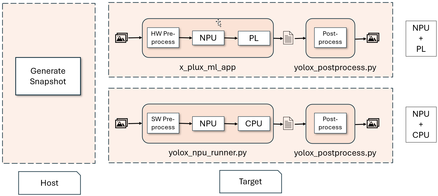
Use the Vitis-AI Docker to generate a snapshot of the YOLOx model specifically for the VEK280 hardware.
Run the following commands on host machine to set up the environment and ensure a snapshot is created for performance IP:
```
source npu_ip/settings.sh VE2802_NPU_IP_O00_A304_M3
```

Generate the snapshot using the following command, run from the root directory of the Vitis-AI repo:

./docker/run.bash --acceptLicense -- /bin/bash -c "source npu_ip/settings.sh && cd /home/demo/YOLOX && VAISW_SNAPSHOT_DUMPIOS=5 VAISW_SNAPSHOT_DIRECTORY=$PWD/yolox.b1 VAISW_RUNOPTIMIZATION_DDRSHAPE=N_C_H_W_c VAISW_QUANTIZATION_NBIMAGES=1 ./run assets/dog.jpg m --save_result"

The generated snapshot directory ($PWD/yolox.b1) from the previous command contains 2 graphs:
- wrp_network_iriz.onnx (NPU graph)
- wrp_network_CPU.onnx (Tail graph for FPGA execution)

Transfer the generated snapshot directory to the VEK280 board, which has been pre-flashed with the reference design image that includes the “yolox_tail” PL kernel.
Copy the dog.jpg file from /home/demo/YOLOX/assets path inside the docker, to VEK280 board.

Use x_plus_ml_app to run the entire workflow. This tool reads the PL kernel information from a JSON file and coordinates the NPU and PL execution.

Preprocessing:
- x_plus_ml_app accepts a JPEG image and preprocesses it using “image_processing” PL IP.
- Set VAISW_RUNSESSION_SUMMARY=all environment variable to enable the performance statistics:
```
export VAISW_RUNSESSION_SUMMARY=all
```

Run the following commands to get the performance numbers.

source /etc/vai.sh
# Below command saves the out in /tmp/app_hls_output0_0_1446_iriz_to_onnx_1_snap_0.bin
x_plus_ml_app -i dog.jpg -c /etc/vai/json-config/yolox_pl.json -s yolox.b1 -r 1

# and run below command, which repeasts NPU+PL for 5 times
x_plus_ml_app -i dog.jpg -c /etc/vai/json-config/yolox_pl.json -s yolox.b1 -m 5

NPU Execution:
- The preprocessed image is processed by the NPU, generating native outputs for the tail graph PL.
PL Execution:
- The PL kernel (yolox_tail) processes the NPU’s output, ensuring high-precision computation and generating results identical to the ONNX graph.

Use yolox_npu_runner.py to run the entire workflow. This tool uses VART.py to read the model input/output information from the snapshot and coordinate the NPU and ONNX execution.

Preprocessing:

The Python app accepts a JPEG image and preprocesses it using Python libraries.

# install onnxrunntime if not already installed
pip3 install onnxruntime==1.20.1

# install PIL for image
pip3 install Pillow

source /etc/vai.sh

VAISW_USE_RAW_OUTPUTS=1 python3 /usr/bin/yolox_npu_runner.py --snapshot yolox.b1 --image dog.jpg --dump_output --num_inferences 5

NPU Execution:
- The preprocessed image is processed by the NPU, generating native outputs for the ONNX graph.
ONNX Graph Execution on CPU:
- The onnxruntime is used to process the NPU’s output on the CPU, providing high-precision computation and generating results.

Output files from the x_plus_ml_app (NPU+PL) and yolox_npu_runner (NPU+CPU) are saved in the following locations for validation: /tmp/app_hls_output0_0_1446_iriz_to_onnx_1_snap_0.bin and /tmp/yolox_output0_0.raw, respectively.
The reference image comes with the yolox_postprocess.py app, which takes dumped outputs from the previous applications and performs post-processing, displaying the results on screen.
The saved files are post-processed using the Python application yolox_postprocess.py, which also takes the original JPG image as input and overlays the detection results over it.

Please install the following packages on the board before running the app:

pip3 install torch
pip3 install torchvision
pip3 install onnx
pip3 install onnxruntime==1.20.1

Run the following script (part of the reference design) to validate and post-process the outputs:

python3 /usr/bin/yolox_postprocess.py --pred_data /tmp/app_hls_output0_0_1446_iriz_to_onnx_1_snap_0.bin --image dog.jpg
python3 /usr/bin/yolox_postprocess.py --pred_data /tmp/yolox_output0_0.raw --image dog.jpg

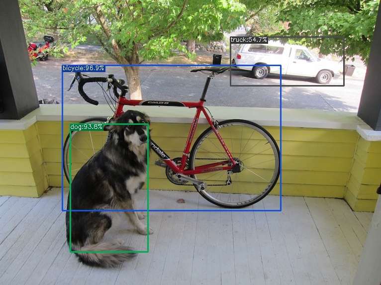
The post-processed results are displayed on the console and also drawn on the input image, saved as the final output (dog_out.jpg).

The console output and annotated output is:

Detection: x0; 125, y0: 132, x1: 565, y1: 424, class: bicycle:96.9%
Detection: x0; 141, y0: 255, x1: 301, y1: 504, class: dog:90.8%
Detection: x0; 464, y0: 73, x1: 699, y1: 174, class: truck:54.7%
Wrote output in:  dog_out.jpg

Performance Comparison#

Following is a performance comparison between the NPU+PL and NPU+CPU configurations for YOLOx inference on the VEK280 hardware. The following numbers do not include the preprocessing and postprocessing.

Metric	NPU+PL	NPU+CPU	Gain
Average Total NPU graph execution time (5 Frames)	(NPU) 3.76 ms	(NPU) 3.80 ms
Average Total tail graph execution time (5 Frames)	(PL) 1.06 ms	(CPU) 21.53 ms	~20 x
Average Total Inference Time (Sequential flow) (5 Frames)	(NPU+PL) 4.82 ms	(NPU+CPU) 25.33 ms	~5 x

This demonstrates the advantage of the hybrid NPU+PL approach, which combines speed and accuracy while reducing CPU workload.

Conclusion#

This approach ensures the system achieves an optimal balance of speed and accuracy:

Speed: NPUs efficiently execute the bulk of computations.
Accuracy: PL handles tasks that demand high precision without burdening the CPU.

By leveraging this hybrid execution model, the X+ML system optimizes performance for AI workloads while meeting the precision requirements of critical tasks.

Optimizing YOLOx Execution with NPU and PL on VEK280 Hardware

Contents