NPU insights#
This section is comprised of five panes: Summary, Original Graph, Optimized Graph, Mapped Graph and Memory Map.
Summary#
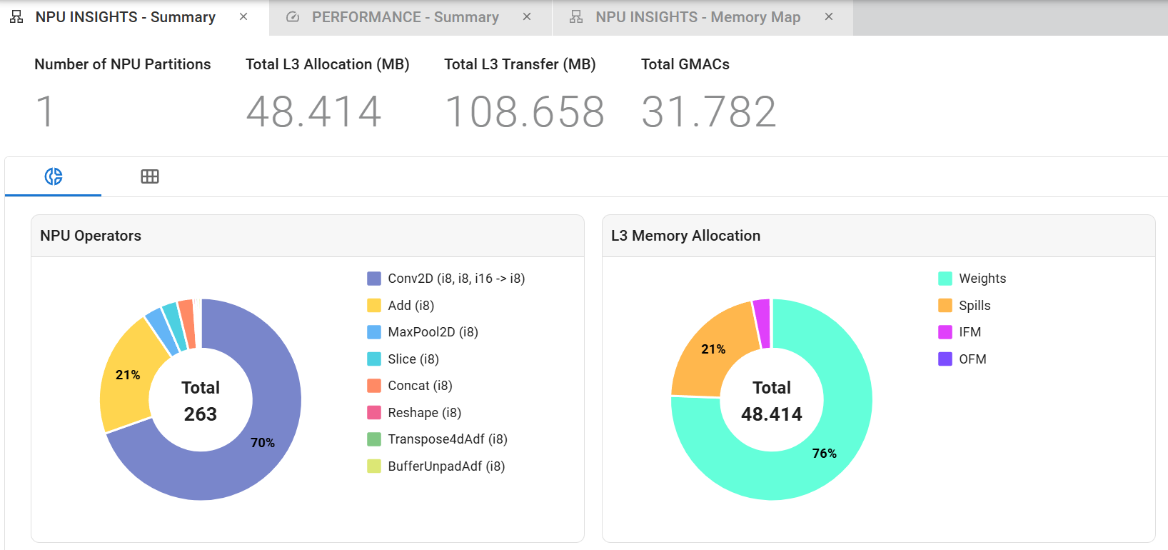
The Summary pane gives an overview of how your model was mapped to the AMD NPU. Number of NPU partitions and Total GMACs mapped to the NPU are displayed, as well as the total L3 memory footprint of the model and the total L3 transfers that is an indication of the amount of data transferred between L3 and L2 memory for the initial input feature map (IFM), the last output feature map (OFM), the weights (WTS) and the spills. Charts are displayed showing statistics on the number of operators in the NPU with their datatypes and L3 Memory Allocation. The L3 Memory Allocation chart shows the distribution of the model’s memory footprint across different L3 memory types (for example, weights, input feature maps, output feature maps and spills). This information can be used to identify potential bottlenecks in the model’s performance and to guide further optimizations. For example, if a large portion of the model’s memory footprint is allocated to weights, it might be beneficial to explore techniques for reducing the size of the weights or optimizing their access patterns.
Original Graph#
This is an interactive graph representing your model, lowered to supported NPU primitive operators and divided into partitions if necessary. As with the PARTITIONING graph, a companion table lists all model elements and supports cross-probing with the graph view. The objects in both the graph and the table also cross-probe with the PARTITIONING graph.
Toolbar#
You can choose to show or hide individual NPU partitions, if any, with the “Filter by Partition” button.
A panel that displays properties for selected objects can be shown or hidden using the “Show Properties” toggle button.
A code viewer showing the MLIR source code with cross-probing can be shown or hidden through the “Show Code View” button.
The following table can be shown and hidden using the “Show Table” toggle button.
Display options for the graph can be accessed with the “Filter Graph” button.
Optimized Graph#
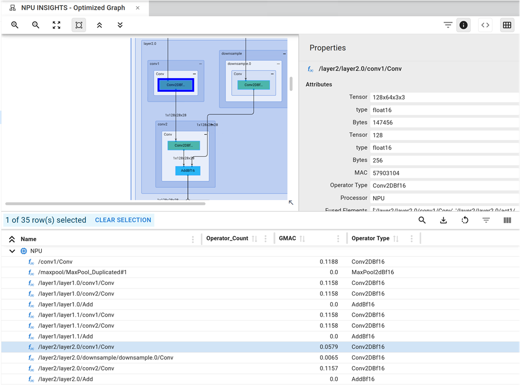
This pane shows the final model that is optimized for the NPU after all transformations and optimizations such as fusion and chaining. It also reports the operators that had to be moved back to the CPU through the Failsafe CPU mechanism. As usual, there is a companion table that follows, containing all of the graph’s elements, and cross-selection is supported to and from the PARTITIONING graph and the Original Graph.
Toolbar#
You can choose to show or hide individual NPU partitions, if any, with the “Filter by Partition” button.
A panel that displays properties for selected objects can be shown or hidden using the “Show Properties” toggle button.
The following table can be shown and hidden using the “Show Table” toggle button.
Display options for the graph can be accessed with the “Filter Graph” button.
Mapped Graph#
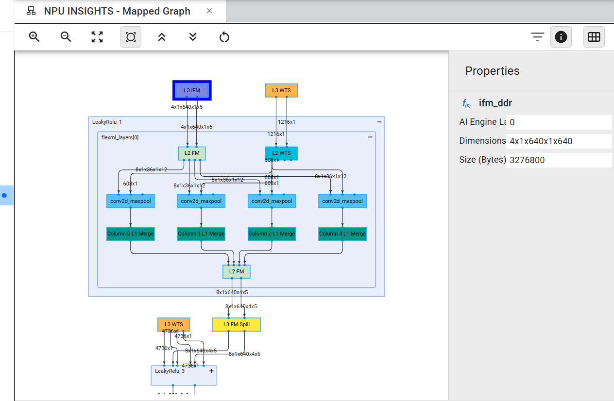
This pane displays the final model mapped to the NPU, including data transfers and memory partitioning required to fit within the device’s memory constraints. The companion table that follows supports cross-selection with the graph visualization, and the properties panel on the right can be toggled for visibility.
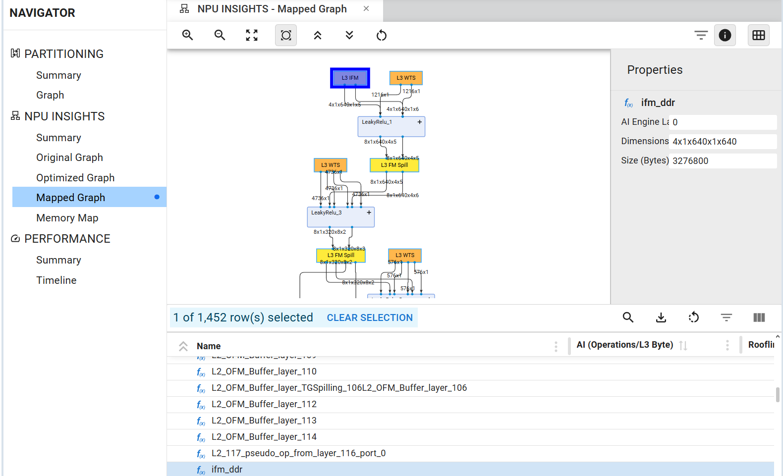
This view provides detailed insights into the hardware implementation. All data transfers from external L3 memory are clearly visible, which consistently occur for weights (WTS) and the initial input feature map (IFM), as well as for intermediate storage operations indicated by the yellow L3 FM Spill boxes.
Expanding the layer boxes reveals the kernel name used within the AI Engine and the number of columns in the graph is the number of columns in the AI Engine Array.
Toolbar#
Filter Graph: Access display options for the graph visualization
Show Properties: Toggle the properties panel for selected objects
Show Table: Toggle the visibility of the data table
Table Toolbar#
Search: Display a search box to locate specific layers or kernels in the table
Export to CSV: Save the table data in CSV format
Reset Settings: Restore table display settings to default view
- Display Modes: Configure table visualization in the following ways:
Block: Displays blocks as they appear in the collapsed graph view
Operator: Displays a detailed view corresponding to the expanded graph
Port: Displays all kernel ports, including DMA ports (feature maps and weights to/from DDR) and RTP ports (kernel parameterization)
- Column Types: Available columns vary depending on the selected element (Block, Operator or Port):
Name: Element identifier
AI (Operations/L3 byte) (Block): Number of operations performed per L3 byte received
Roofline (Operations/Cycle) (Block): Maximum number of operations the block can perform based on memory bandwidth and hardware compute capacity
Type (Operator): Operator classification—either data manipulation (external buffer, shared buffer, packet merge, or packet split) or function
Function (Operator): For function-type operators, displays the hardware function name
Tiling (Port): Indicates the size of blocks transmitted through the DMA (maximum 5D blocks)
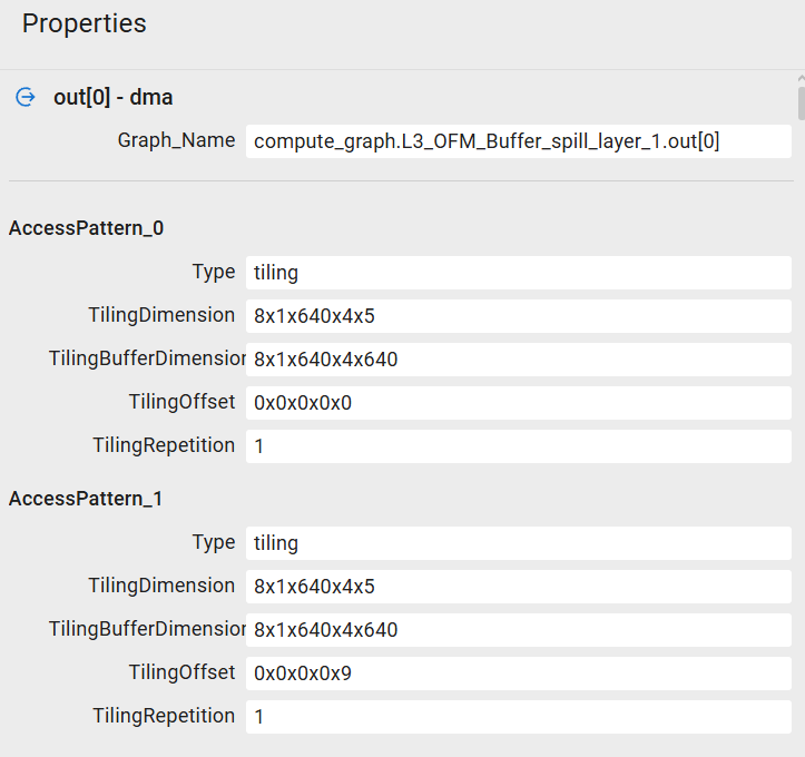
Note
For DMA operations, the Properties panel displays tiling information showing how buffer data is partitioned and transmitted through the DMA channel. In the screenshot below, the buffer represents a memory space of 13,107,200 pixels, logically organized according to the Tiling Buffer Dimension parameter: 8x1x640x4x640 (640 columns, 4 rows, 640 channels, etc.). AccessPattern_0 indicates that a single 5D tile (Tiling Repetition) of size 8x1x640x4x5 (Tiling Dimension) is extracted from the buffer space, starting at offset 0x0x0x0x0 (Tiling Offset). Subsequent tiles are extracted as described in AccessPattern_1 and beyond.
Data Parallelism Visualization#
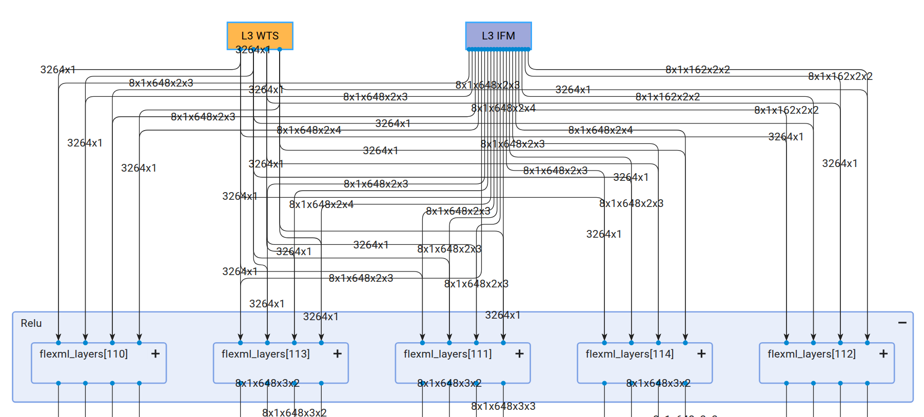
Data Parallelism is a technique that enables concurrent processing of multiple input samples on the NPU through replication of the fundamental NPU Compute Unit. In this configuration, all input samples are processed synchronously across all NPU in a layer-by-layer fashion. This approach enables users to enhance NPU throughput, albeit with increased resource utilization. The following figure illustrates an implementation with 6 replicated instances of the base NPU Compute Unit, allowing for the concurrent processing of 6 input samples:
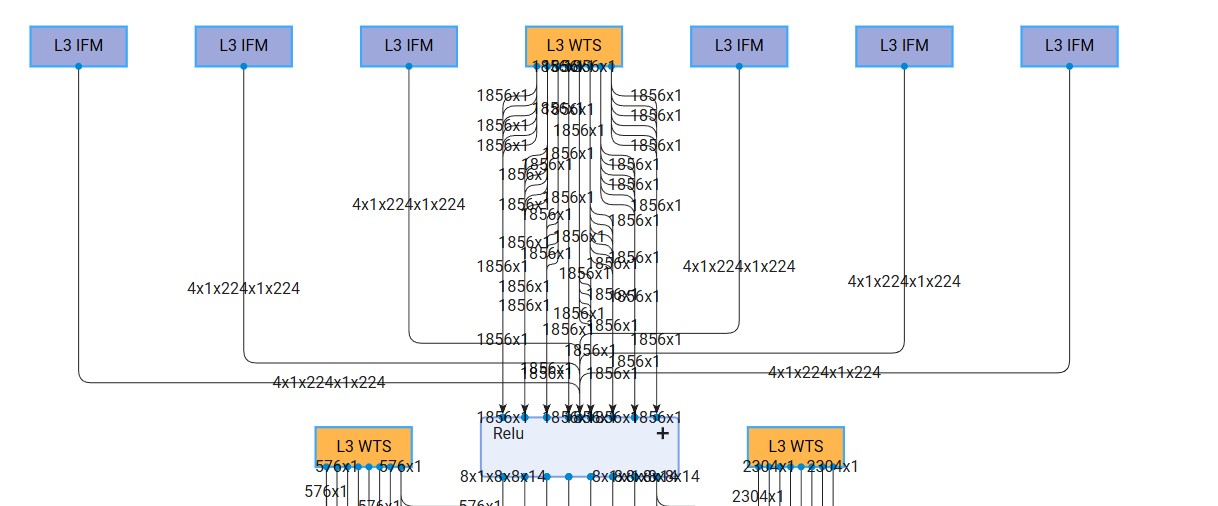
Upon expanding the first layer, it becomes evident that each input sample is processed by a dedicated instance of the fundamental NPU Compute Unit.
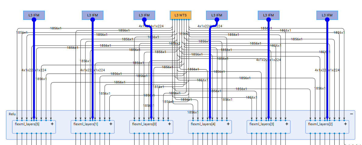
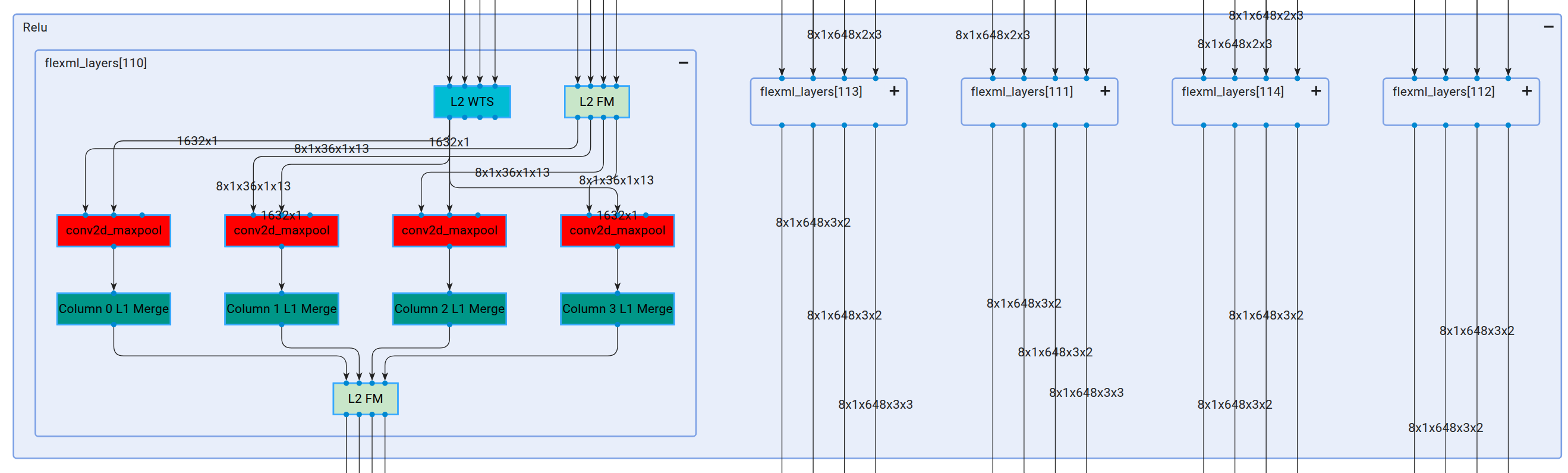
Further expansion of an individual overlay reveals the underlying 4-column architecture characteristic of the basic NPU configuration.
A key architectural advantage of this design is the utilization of a single weight DMA channel to supply data to all NPU Compute Units.
This consolidation significantly reduces communication overhead between the DDR memory and the AI Engine-ML array.
Tensor Parallelism Model Visualization#
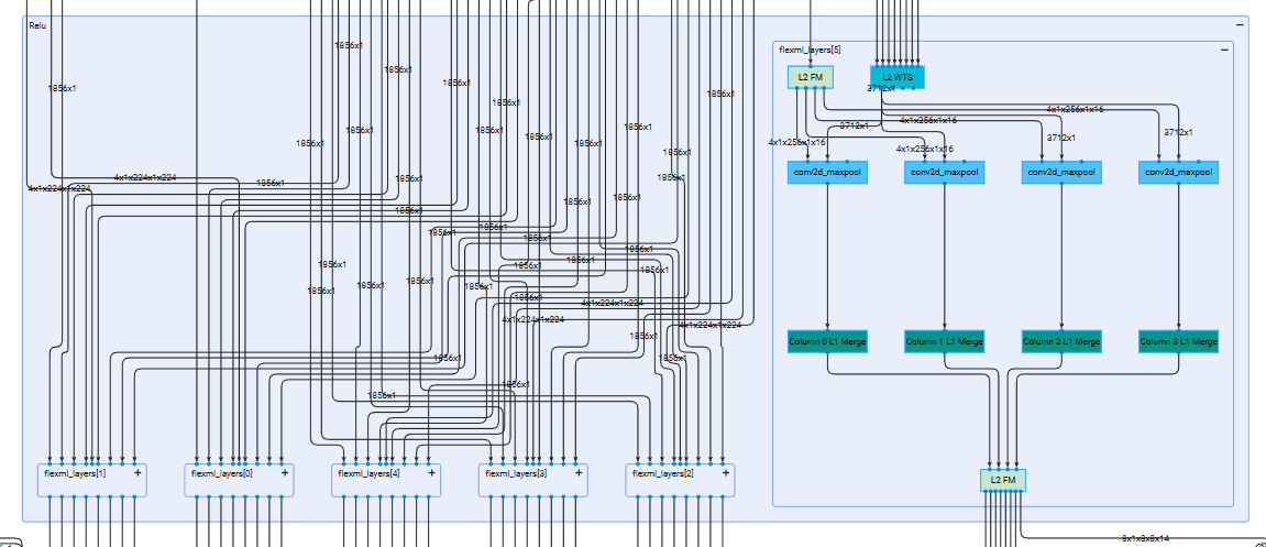
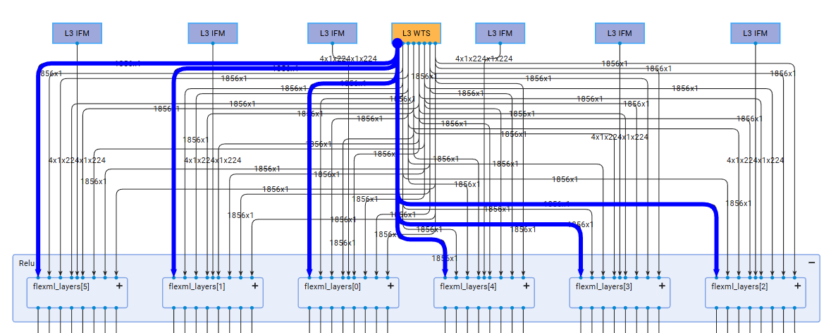
Tensor Parallelism is a technique that distributes the processing of a single input sample across multiple instances of the NPU Compute Units. At each layer, the Input Feature Map (IFM) is partitioned across all instances, thereby reducing overall latency. The following figure demonstrates a model implementation optimized for latency:
The diagram shows that a single IFM is distributed across 5 NPU Compute Units. Upon further expansion of these instances, each is revealed to comprise 4 columns:
Memory Map#
This pane illustrates how model data—including input and output feature maps (IFM, OFM) and weights (WTS)—are mapped to memory on a layer-by-layer basis. For L2 memory (Memory Tile of the AI Engine Array), the exact location and size are displayed as defined during compilation. For L3 memory, only the footprint of IFM, OFM, and weights is shown.
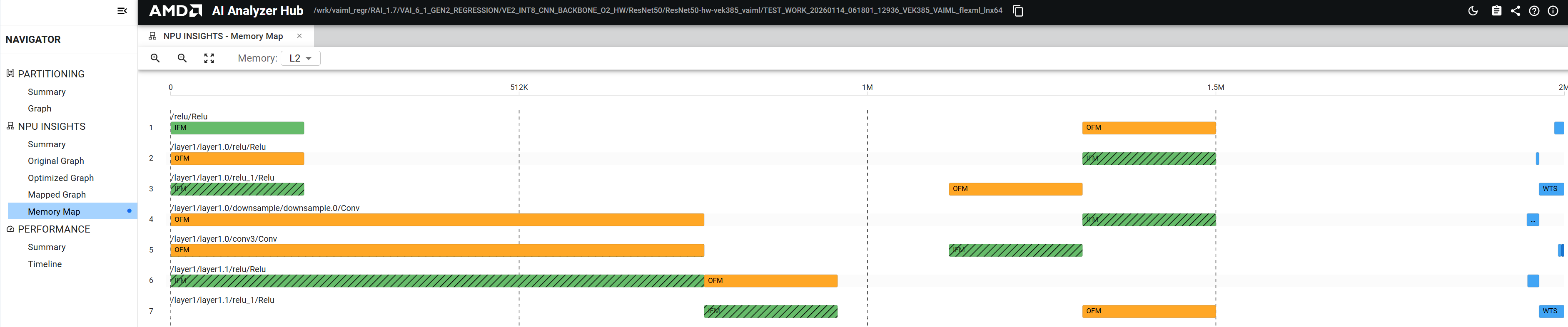
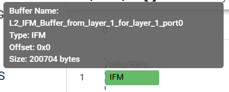
IFMs are represented as green boxes, OFMs as orange boxes, and WTS as blue boxes. Light and dark shading indicates ping-pong buffering. Hovering over any box displays a tooltip with the buffer name, data type, memory offset, and buffer size.
The memory span appears at the top of the map. This visualization facilitates understanding of data transfers throughout the device, enabling identification of performance bottlenecks. For example, a hashed pattern on an IFM box indicates that the data was already resident in memory as the OFM of a previous layer.
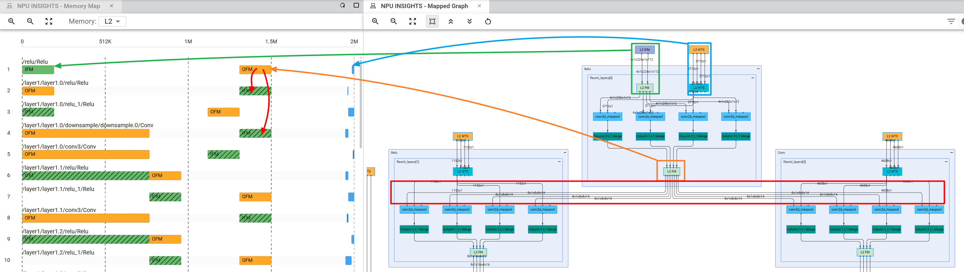
In the screenshot below, the memory map and mapped graph are displayed side by side. The first IFM originates from DDR (L3 memory) and is shown as a solid green box. Weights (WTS) always originate from DDR and are consistently displayed as solid blue boxes. After the OFM is computed, the data is reused as the IFM for both the second and fourth layers, indicated by the hashed pattern on these IFMs.
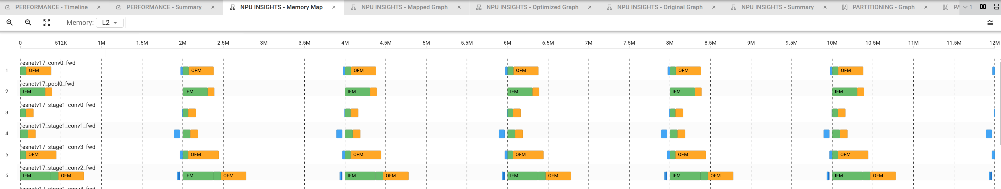
When multiple 4x4 base blocks are used in parallel for either data or tensor parallelism, the memory map provides insights into how data is distributed across the different instances. For example, in a latency optimized graph where 6 instances are used in parallel, the memory map reveals that the IFM is partitioned across all 6 instances, while the weights are shared among them. This visualization helps users understand the data flow and memory usage patterns in their model, enabling them to make informed decisions about further optimizations.
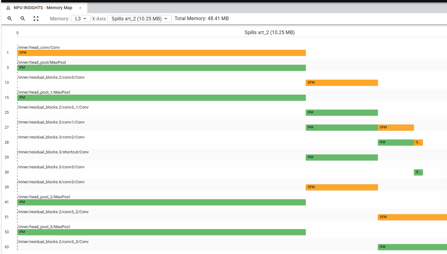
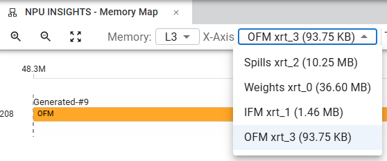
Displaying L3 Memory map (DDR) is also possible. The exact location of data in L3 memory is not defined during compilation and can vary between inferences. However, the overall footprint of IFMs, OFMs, weights and spills of L2 memory can be observed in L3 memory. The following screenshot shows how to select between the various elements to display in L3 memory:
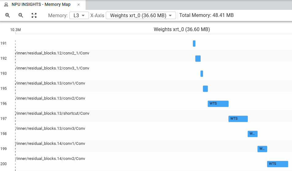
L2 spills to L3 memory and Weights stored in L3 memory are given layer by layer in the memory map, allowing you to understand the data transfers between L3 and L2 memory as well as the relative size of the weights.
In the screenshot below we can see that the weights are stored in non overlapping contiguous memory spaces:
In the following screenshot we can see the L3 memory footprint of L2 spills. Spilling being temporary by nature, the spilled data for different layers can be located in overlapping memory spaces in L3 memory: