Data Parallelism and Tensor Parallelism#

Overview#

The VAIML Compiler provides two parallelization strategies to optimize model performance. Understanding when to apply each approach is essential for achieving your performance goals.

Data parallelism instantiates the entire model multiple times across the device through replication of the NPU compute unit. With dp_size=4, four independent model instances process different inference requests simultaneously. Each input sample is processed by a dedicated NPU compute unit instance, and all instances execute synchronously in a layer-by-layer fashion. The advantage of this approach is that all replicated instances share a single weight DMA channel, reducing communication overhead between DDR memory and the AI Engine array. Use this approach when you need to maximize throughput for concurrent requests, such as processing multiple camera streams in a video analytics application.

Tensor parallelism partitions a single inference request across multiple NPU compute units. With tp_size=4, the computation for one request is divided into four parallel execution streams, reducing the time required to complete that request. This approach is appropriate when minimizing per-request latency is critical, or when the model’s memory requirements exceed the capacity of a single NPU compute unit.

Hardware Terminology#

Understanding the hardware organization is essential for configuring parallelism:

AIE tile: A single processing element in the AI Engine. This is the smallest hardware unit that executes model operations.
NPU compute unit: A rectangular group of AIE tiles. For ve2-xc2ve3558 and ve2-xc2ve3858 devices, each compute unit consists of 4×4 = 16 AIE tiles.
AIE array: The complete rectangular grid of AIE tiles on the device. For example, ve2-xc2ve3558 has a 4 rows × 24 columns array (96 total tiles).
NPU columns: The vertical columns in the AIE array.

Compiler Options#

Data Parallelism (dp_size)#

The dp_size parameter (default: 1) controls the number of model instances through replication of the base NPU compute unit. Setting dp_size=6 creates six identical instances of your model, each capable of processing a separate inference request. All instances process their inputs synchronously, progressing through the model layer-by-layer in lockstep. Higher values increase concurrent request handling capacity.

Tensor Parallelism (tp_size)#

The tp_size parameter (default: 0) controls how computation is distributed within a single inference request. Setting tp_size=4 partitions the model’s operations across four NPU compute units through a technique called sharding. Each NPU compute unit handles a portion of the input data in parallel.

When set to 0, the compiler automatically selects an appropriate tp_size value based on the target device characteristics and model requirements. Note: The value 0 is a special sentinel flag that triggers auto-selection; it is not used as a literal multiplier in resource calculations. After compilation, the compiler resolves this to a concrete value. This automatic selection provides a reasonable default for most use cases.

Tensor parallelism serves two primary purposes: reducing per-request latency through parallel execution, and enabling deployment of models whose memory footprint exceeds a single NPU compute unit’s capacity.

Setting Compiler Options#

Specify dp_size and tp_size in the vitisai_config.json configuration file under the vaiml_config section:

{
    "passes": [
        {
            "name": "init",
            "plugin": "vaip-pass_init"
        },
        {
            "name": "vaiml_partition",
            "plugin": "vaip-pass_vaiml_partition",
            "vaiml_config": {
                "device": "ve2-xc2ve3558",
                "dp_size": 6,
                "tp_size": 1
            }
        }
    ],
    "target": "VAIML",
    "targets": [
        {
            "name": "VAIML",
            "pass": [
                "init",
                "vaiml_partition"
            ]
        }
    ]
}

If not specified, the compiler uses default values: dp_size=1 (no data parallelism) and tp_size=0 (automatic tensor parallelism selection).

Device Constraints and Resource Usage#

Valid Configuration Ranges:

The product of dp_size × tp_size is limited by the device hardware. Common configurations:

Device	Common dp_size × tp_size values	AIE array (rows × columns)
ve2-xc2ve3558	Up to 6 (for example, 6×1, 3×2, 2×3, 1×6)	4 rows × 24 columns (96 tiles)
ve2-xc2ve3858	Up to 9 (for example, 9×1, 3×3, 1×9)	4 rows × 36 columns (144 tiles)

Resource Calculation:

Each configuration consumes AIE tiles according to this formula:

AIE tiles used = dp_size × tp_size × NPU_compute_unit_size

Where NPU_compute_unit_size is the number of AIE tiles per compute unit, which depends on the device. For ve2-xc2ve3558 and ve2-xc2ve3858 devices, each NPU compute unit uses 4×4=16 AIE tiles.

Note: This formula applies only when tp_size ≥ 1. When tp_size=0 (auto-select), the compiler first resolves it to a concrete value before calculating resource usage.

For example (on devices with 16 tiles per compute unit): - dp_size=3, tp_size=2: uses 3 × 2 × 16 = 96 AIE tiles - dp_size=4, tp_size=1: uses 4 × 1 × 16 = 64 AIE tiles

Note: Some devices use different compute unit sizes (for example, 2×4=8 tiles per unit). The calculation method remains the same.

The compiler maps your chosen dp_size and tp_size to the available hardware automatically. If your configuration exceeds device capabilities, compilation fails with an error.

Visualizing Data and Tensor Parallelism#

The following diagram illustrates how dp_size=2 and tp_size=2 work together. When you send 2 inference requests at runtime, each is processed by a separate model instance (using data parallelism), and within each instance, the computation is sharded across 2 NPU compute units (using tensor parallelism).

With tensor parallelism, at each layer of the model, the input activations are partitioned across the tensor parallelism shards (TP 0, TP 1, etc.), allowing parallel processing that reduces overall latency

../../_images/X60254-runtime_batches.png

Two Inference Requests Arrive at Runtime
┌─────────┐  ┌─────────┐
│Request 1│  │Request 2│
└────┬────┘  └────┬────┘
     │            │
     │            │          Data parallelism (dp_size=2)
┌────▼────────────▼────┐    2 model instances process requests in parallel
│                      │
│  ┌───────────────┐   │
│  │Model Instance0│   │    Processes Request 1
│  │  ┌─────┬─────┐│   │
│  │  │TP 0 │TP 1 ││   │    Tensor parallelism shards (tp_size=2)
│  │  │ ½   │ ½   ││   │    Input activations partitioned across 2 shards
│  │  │acts │acts ││   │
│  │  └─────┴─────┘│   │
│  └───────────────┘   │
│                      │
│  ┌───────────────┐   │
│  │Model Instance1│   │    Processes Request 2
│  │  ┌─────┬─────┐│   │
│  │  │TP 0 │TP 1 ││   │    Tensor parallelism shards (tp_size=2)
│  │  │ ½   │ ½   ││   │    Input activations partitioned across 2 shards
│  │  │acts │acts ││   │
│  │  └─────┴─────┘│   │
│  └───────────────┘   │
└──────────────────────┘

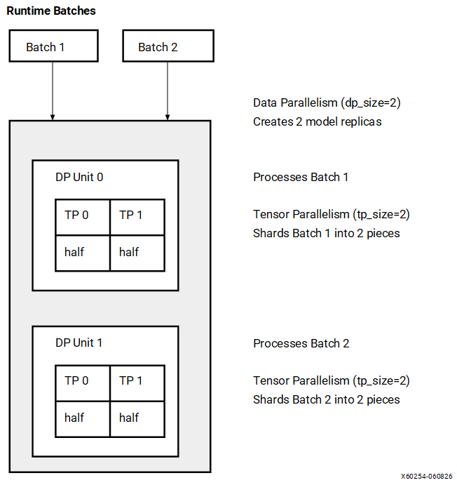
Legend:
- TP 0, TP 1: Tensor parallelism shards (partitions of the computation)
- ½ acts: Half of the input activations processed at each layer

Configuration: dp_size=2, tp_size=2
AIE tiles used: 2 × 2 × 16 = 64 tiles (on devices with 16 tiles/compute unit)

Key observations:

Data parallelism: 2 model instances process different inference requests simultaneously. The instances execute synchronously in a layer-by-layer fashion, and share a single weight DMA channel to reduce DDR memory bandwidth overhead.
Tensor parallelism: Within each instance, computation is split across 2 NPU compute units to reduce latency. At each layer, input activations are partitioned across the tensor parallelism shards.
Total AIE tiles: 2 × 2 × 16 = 64 tiles (each compute unit uses 4×4=16 tiles on these devices)

Choosing Your Configuration#

The choice between data and tensor parallelism depends on your performance requirements:

Prioritize dp_size for throughput-oriented workloads. Applications that process multiple concurrent requests—such as batch image processing pipelines, multi-camera surveillance systems, or API services—benefit from higher dp_size values. Each model instance processes one request independently, so dp_size=6 enables six simultaneous requests. See Architectural Comparison: Single Instance (dp_size > 1) vs. Multi-Instance (dp_size = 1) for performance considerations on memory-bound models.

Prioritize tp_size for latency-sensitive workloads. Real-time applications where per-request processing time is critical benefit from higher tp_size values. Setting tp_size=6 distributes a single request’s computation across six NPU compute units, reducing completion time. This allocation dedicates more hardware resources to each request, limiting concurrent request capacity.

Combining both parameters (dp_size > 1 and tp_size > 1) addresses workloads requiring both throughput and low latency. For example, dp_size=2, tp_size=3 creates two model instances, each using three-way parallelism. This configuration handles two concurrent requests with reduced per-request latency, at the cost of increased hardware resource consumption.

Default configuration: If dp_size and tp_size are not specified, the compiler uses the following default values:

dp_size: 1
tp_size: 0 (automatic selection)

When tp_size is set to 0, the compiler automatically selects an appropriate value during compilation. For the ve2-xc2ve3858 device, the compiler selects the optimal distribution of compute resources, up to a maximum of 6x4 columns.

Recommended Configurations for `ve2-xc2ve3858`#

The following configurations are recommended depending on your performance requirements:

Optimization Goal	`dp_size`	`tp_size`
Optimal utilization	6	1
Balanced latency and utilization	3	2
Optimal latency and utilization	1	6

Configuration Examples#

The following table shows common configurations for different performance objectives. You can choose other values based on your specific requirements and device capabilities.

Device	dp_size	tp_size	AIE Tiles Used	Use Case
ve2-xc2ve3558	6	1	96	High throughput: 6 requests processed concurrently
ve2-xc2ve3558	3	2	96	Balanced: 3 requests concurrently, each with 2-way parallelism
ve2-xc2ve3558	1	6	96	Low latency: Each request parallelized across 6 units
ve2-xc2ve3858	9	1	144	High throughput: 9 requests processed concurrently
ve2-xc2ve3858	3	3	144	Balanced: 3 requests concurrently, each with 3-way parallelism
ve2-xc2ve3858	1	9	144	Low latency: Each request parallelized across 9 units

Runtime Request Handling#

The dp_size configuration does not limit the total number of inference requests you can submit. When the number of incoming requests exceeds the available model instances, the runtime queues requests and processes them in multiple rounds.

For example, with dp_size=4:

16 requests: Processed in 4 rounds of 4 requests each
15 requests: Processed in 3 full rounds (12 requests) plus a fourth round with 3 requests. The AMD Vitis™ AI Execution Provider pads the final round to 4 requests using inputs padded with zeros for efficient execution and returns only outputs from the real requests.

This means dp_size affects throughput and latency characteristics, but does not impose a hard limit on request volume. The runtime automatically manages request queuing and scheduling across available model instances.

Application Scenarios#

Example 1: High-Throughput Image Processing

A cloud-based image processing service handles hundreds of concurrent user requests during peak hours. Latency requirements are moderate, but the system must maximize throughput.

For this workload on ve2-xc2ve3558, configure for high throughput using data parallelism:

"vaiml_config": {
    "device": "ve2-xc2ve3558",
    "dp_size": 6,
    "tp_size": 1
}

This configuration creates six independent model instances. The runtime distributes incoming requests across all instances, maximizing concurrent request processing. Individual request latency matches the single-instance baseline, but aggregate throughput scales with the number of instances.

Example 2: Low-Latency Real-Time Inference

A real-time video processing application requires low inference latency for smooth user experience. The application processes a single video stream, making throughput less critical than per-frame latency.

For this workload, configure for low latency using tensor parallelism:

"vaiml_config": {
    "device": "ve2-xc2ve3558",
    "dp_size": 1,
    "tp_size": 6
}

This configuration partitions the model across six processing units. Each inference request leverages all six units executing in parallel, reducing per-request completion time. The system can process only one request at a time, but completes each request faster than the baseline configuration.

Example 3: Multi-Camera Automotive System

An automotive perception system processes four camera streams simultaneously (front, rear, left, right). Each camera requires consistent frame-to-frame latency for reliable object detection. All streams must be processed concurrently in real-time.

This workload maps naturally to data parallelism with one model instance per camera:

"vaiml_config": {
    "device": "ve2-xc2ve3558",
    "dp_size": 4,
    "tp_size": 1
}

Each model instance processes one camera stream independently. When frames arrive from all cameras simultaneously, all four instances execute in parallel, providing consistent latency across cameras.

This configuration consumes 4 × 1 × 16 = 64 AIE tiles from the 96 tiles available on ve2-xc2ve3558, representing 67% utilization. The remaining capacity allows scaling to dp_size=6 if additional camera streams are required.

Running Multiple Models Concurrently#

The configurations described in this guide apply to single-model deployments. Applications requiring multiple models to execute concurrently on the same device must use multi-tenancy capabilities.

Multi-tenancy enables resource sharing between models through two mechanisms:

Spatial sharing allocates different NPU column ranges to each model, enabling true parallel execution without interference.

Temporal sharing time-multiplexes multiple models on the same NPU columns. This approach is necessary when combined resource requirements exceed available hardware, with the trade-off of context-switching overhead.

For example, on ve2-xc2ve3558, you can run a 4-camera perception model (dp_size=4, tp_size=1, 64 tiles) alongside a traffic sign classifier (dp_size=1, tp_size=1, 16 tiles). Each model is compiled with its own dp_size and tp_size configuration. Runtime column allocation is then configured using start_column and aie_columns_sharing parameters.

For runtime placement, spatial zones, and temporal sharing, see Multi-Tenancy: Spatial and Temporal Sharing.

Optionally, when the compiled model is deployed, the runtime output can indicate how many columns are used on the NPU. Add the following configuration to the xrt.ini file in the working directory on the board where you run the inference:

[Runtime]
verbosity=7

After running inference, a message similar to the following indicating the column usage appears:

[xrt_xdna] DEBUG: Partition Created with start_col 0 num_columns 20 partition_id 5120

Alternatively, you can probe the runtime status while inference is running on the board using the following command:

xrt-smi examine --device 0 --report aie-partitions

This command displays the column usage for each process. For an example of the output, see XRT-SMI Utility.

Architectural Comparison: Single Instance (dp_size > 1) vs. Multi-Instance (dp_size = 1)#

When deploying parallel inference on identical total NPU hardware resources (for example, a 4×4 array of compute units), you can structure your host application in two distinct configurations:

Single instance (dp_size>1): A single host application thread drives a single compiled model instance, batching multiple requests together (for example, dp_size=4 driven by a single application thread).
Multiple instances (dp_size=1): Multiple independent host applications (or threads) each run a separate, dedicated model instance on their own assigned compute units.

While both configurations consume the exact same number of AIE tiles and execute the same per-request computations, they can produce noticeably different end-to-end throughput. The difference comes from how each approach drives DDR bandwidth, not compute efficiency.

Why Performance Varies by Configuration

In a single dp_size>1 instance, the batches execute in lock-step. All batches enter the same layer at the same time, so the bandwidth demand of memory-heavy layers (large weights, large activations) is aligned in time. The instantaneous DDR bandwidth requirement becomes roughly N × peak where N is the batch count. When this peak exceeds the available DDR bandwidth, the NPU stalls waiting for memory.

In a multi-instance dp_size=1 configuration, each instance runs independently. Operating system thread scheduling naturally introduces minor phase offsets (sub-millisecond stagger) between instances. As a result, the instances rarely hit memory-heavy layers at the exact same time, and the aggregate bandwidth demand curve is smoothed out. This typically yields better DDR utilization and higher overall throughput on memory-bound models.

Configuration Selection Criteria

Selecting the correct deployment configuration depends on your model’s resource utilization profile, host architecture constraints, and latency requirements. Use the guidelines below to determine whether to deploy a single batched instance or multiple independent instances.

Guidelines for Single-Instance Deployment (dp_size > 1)

Select a single-instance configuration with a batch size greater than 1 if your deployment meets the following criteria:

Compute-Bound Workloads: The model architecture exhibits high arithmetic intensity (high MAC utilization) where peak DDR memory bandwidth is not the primary performance bottleneck.
Streamlined Programming Model: The application design favors lower complexity, utilizing a single application context and a single inference call to process multiple concurrent requests.
Synchronized Output Requirements: The downstream application logic requires deterministic, synchronized batch completion, meaning all parallel outputs must be available at the exact same execution boundary.
Host Resource Constraints: The host system environment or application architecture cannot easily manage or scale multiple concurrent runtime threads or processes.

Guidelines for Multi-Instance Deployment (dp_size = 1)

Select a multi-instance configuration with independent, single-batch models if your deployment meets the following criteria:

Memory-Bound Workloads: The model architecture is constrained by memory transfers, and DDR bandwidth saturation is the dominant bottleneck preventing maximum hardware efficiency.
Maximum Aggregate Throughput Priority: The primary deployment goal is maximizing total system processing volume over time, and the application can tolerate minor variations in per-request latency.
Naturally Disjoint Data Streams: The ingestion pipeline inherently handles isolated data channels—such as independent multi-camera feeds or multi-tenant network requests—that map cleanly to separate execution contexts.
Asynchronous Execution Progress: Each incoming request stream must make independent forward progress through the NPU without being blocked by global synchronization points or waiting for neighboring batches to complete.

Workflow Recommendations

Profile the model first: Execute an initial profile of the target model on the reference device. Measure and record both the AIE MAC utilization percentage and the DDR bandwidth utilization levels.
Evaluate Bottlenecks:

If the workload is constrained by memory bandwidth, implement Multi-Instance (dp_size=1).

If the workload is constrained by raw compute cycles, implement Single Instance (dp_size>1) to reduce host-side thread management overhead.
When in doubt, measure both configurations on the target device. Because both configurations leverage identical physical tile layouts, switching between strategies requires only model recompilation and a modification to the host application dispatch logic. Engineers should benchmark both configurations under realistic workloads to validate performance assumptions before production sign-off.

Data Parallelism and Tensor Parallelism

Contents