DDR Throughput Profiling#
This section describes the enhanced profiling options available in AMD Vitis™ AI and explains how to use DDR memory throughput data within AI Analyzer to evaluate the efficiency of data transfers between the L2 [AI Engine Memory Tile] and L3 [DDR] cache levels.
Enabling Enhanced Profiling#
Profiling DDR throughput and cache behavior helps identify where performance is not optimal. AI models are often bottlenecked not by compute, but by memory access inefficiency. The processor is typically waiting on data rather than actively computing.
To collect profiling data, the compiled model must be instrumented before deployment. Instrumentation configures the interfaces between NoC and the AI Engine array to capture the required performance metrics.
Configuration#
Compilation and runtime profiling options are specified in the vitisai_config.json configuration file.
Configuration Example#
    {
"passes": [
    {
        "name": "init",
        "plugin": "vaip-pass_init"
    },
    {
        "name": "vaiml_partition",
        "plugin": "vaip-pass_vaiml_partition",
        "vaiml_config": {
            "device": "ve2-xc2ve3858", # for XC2VE3858
            "keep_outputs": true,
            "log_level": "info",
            "ai_analyzer_enhanced_profiling": [
                "control_instrumentation"
            ],
            "profiling_runtime_config": {
                "control_instrumentation": {
                "interface_tile": "peak_read_bandwidth"
                }
            }
        }
    }
],
"target": "VAIML",
"targets": [
    {
        "name": "VAIML",
        "pass": [
            "init",
            "vaiml_partition"
        ]
    }
]
    }
Important
Before executing the model on hardware, select either read-bandwidth profiling or write-bandwidth profiling. Both metrics cannot be captured simultaneously in a single run. In the previous configuration example, read-bandwidth profiling is enabled through the peak_read_bandwidth interface tile setting. To capture write bandwidth instead, set the interface tile to peak_write_bandwidth.
The DDR memory has a limited capacity for storing timestamps. When running a large number of inferences, the runtime begins overwriting earlier timestamp records once this limit is reached meaning only the most recent timestamps will be available at the end of execution.
Running Model on Hardware#
After compiling the model with the appropriate configuration, run inference on the target hardware. During execution, the runtime automatically generates timestamp files and, for enhanced profiling, trace-dump files containing profiling data for each inference. These files are required for AI Analyzer performance analysis.
Execution and Trace Generation
When the model runs on target hardware, the runtime automatically generates one trace-dump file per inference. During execution, the console also displays informational messages for each inference, such as:
[2026-05-29 09:17:01.684] [console] [info] [FLEXMLRT] ../../flexml_rt/src/FlexMLDispatcher.cpp:1015 hsiSlot OFM iter=0 i=0 b=0 batch_index=0 outSlot=0 layout=batch-major name=compute_graph.ofm_ddr cpu_shape=[1,1000] elements=1000 outNumElem[i]=1000
Trace Dump Files
After inference completes, a set of timestamp files and trace-dump files is generated in the current working directory:
dtrace_dump_ctx_1_run_0_2026-05-29_09-17-01-685212.py  dtrace_dump_ctx_1_run_0_2026-05-29_09-17-10-275761.py
dtrace_dump_ctx_1_run_0_2026-05-29_09-17-03-060857.py  dtrace_dump_ctx_1_run_0_2026-05-29_09-17-12-077385.py
...
record_timer_inference_0xaaaaf344c600_0_281473818165280.json
record_timer_subgraph_cpu_ts.json
record_timer_ts.json
record_timer_vaip_vaiml_par_0.json
Aggregating Profiling Data
AI Analyzer requires all profiling files to be aggregated into a single archive for processing. After inference execution completes, run the following command to collect and package the data:
vaiprofile-collect-data .
This command moves all trace-dump and timestamp files into the vai_profile_dir directory and generates a vai-profile.zip archive from that directory. Transfer this file to your host computer for subsequent analysis with AI Analyzer.
After transferring vai-profile.zip to the host machine, process it with the following command:
vaiprofile <VAIML_design_dir_path> vai_profile.zip --frequency <freqMHz>
Where <freqMHz> is the AI Engine array clock frequency in MHz, for example, 1250 for a 1.25 GHz clock.
The vai_profile.zip archive is extracted into vai_profile_dir, where all included files are processed and the results are stored in a directory named analyzed_data under <VAIML_design_dir_path>. This directory contains processed profiling data that is automatically used when AI Analyzer is launched with the same <VAIML_design_dir_path> as the logdir argument. The data is visualized in the Performance section of AI Analyzer.
There is a last operation to perform before the data is available in AI Analyzer:
cd <VAIML_design_dir_path>
cp analyzed_data/mlprofiler_ddr_merge/record_timer*.json analyzed_data
cp analyzed_data/mlprofiler_ddr_merge/onnxruntime_profile_*.json analyzed_data
Note
The file analyzed_data/mlprofiler_ddr_merge/partition_info.json contains a summary of the partitions that have been profiled with the number of inferences that have been kept in the timestamp files:
 "partition_info": {
  "ctx": {
    "0": {
      "run": {
        "0": {
          "subgraph": "vek385_cache_dir/resnet50-Base/vaiml_par_0/0",
          "work_dir": "/group/techsup/oliviert/Tutorials/TPvsLatency/Resnet50DDR/./vek385_cache_dir/resnet50-Base/vaiml_par_0/0/aiecompiler/Work",
          "total_num_inferences": 2020,
          "num_inferences_in_record_timer": 268
        }
      }
    }
  }
}
In this specific case, out of 2,020 total inferences:
Timestamp data: Only the last 268 inferences are retained in the timestamp files and available for analysis in AI Analyzer.
DDR Bandwidth data: All 2,020 inference files containing DDR bandwidth data remain fully available on disk.
Using Enhanced Profiling DDR Bandwidth Columns#
If model performance is below expectations, use the DDR bandwidth columns to determine whether a memory bandwidth bottleneck is present. If the minimum observed throughput for a layer is significantly below 10 GB/s (for a 1.25 GHz AI Engine array clock), that layer might be limited by memory access.
Use the reported column and channel information to identify where the bottleneck occurs, then verify whether it recurs across multiple layers.
If the same column and channel consistently show low throughput, this may indicate inefficient memory-controller parameterization or issues with AI Engine GMIO parameters. In that case, adjust GMIO parameters using gmio_train Configuring NoC Connectivity for Model Deployments or tune memory-controller settings, then reassess throughput and overall model performance.
DDR Throughput Analysis Methodology#
Purpose#
Memory bandwidth analysis helps determine whether an AI model deployment is:
- Memory-bound
limited by DDR/memory throughput
Enhanced Profiling gives us access to DDR/L2 bandwidth metrics but not L2/L1 data transfers
- Compute-bound
limited by processing capacity
Low Efficiency (%) in AI Analyzer with high DDR bandwidth suggests compute-bound layer.
- Well-balanced
optimal hardware utilization
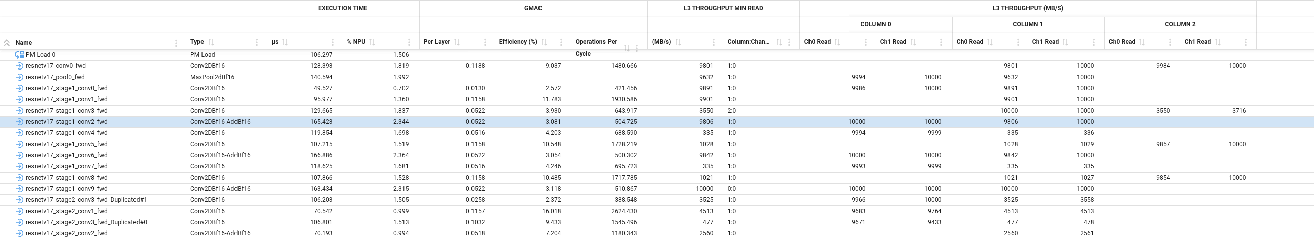
Data is available in the Performance tab of AI Analyzer, including columns for minimum observed DDR read/write throughput (MB/s) per layer and the corresponding column and channel where it occurred. For automated analysis, refer to the instrumentation_stats_ctx_<l>_run_<m>_inf_<m>.json files generated during the vaiprofile step; these files contain the same information in machine-readable form.
Perform this analysis during performance optimization, especially when investigating latency issues or unexpected performance degradation.
Analysing these json files can give you answers to the following questions:
Are there memory bottlenecks limiting performance?
Do different columns:channel experience shared or independent bottlenecks?
Is bandwidth variance expected (heterogeneous workload) or problematic (instability)?
How is workload distributed across memory channels?
Is there room for throughput optimization?
Analyzing NoC-to-AI Engine Throughput Data#
The throughput JSON files capture the memory bandwidth measured between the Network-on-Chip (NoC) and the AI Engine array, recorded at every column and channel of the model. This data can be used to identify potential memory access bottlenecks that might impact model performance.
Throughput Thresholds#
Thresholds can be set in advance; however, interpretation should be based on the specific model and performance goals. The following thresholds are relative to the maximum theoretical bandwidth of 10 GB/s for a 1.25 GHz AI Engine array clock:
~10,000 MB/s (optimal): Full bandwidth utilization — no memory bottleneck
≥ 2,000 MB/s (acceptable): Within acceptable range — monitor for degradation
< 2,000 MB/s (problematic): Potential memory access issue — further investigation required
Pattern Detection and Variance Analysis#
To identify memory access issues, analyze the throughput data across all columns and channels, looking for the following patterns:
Consistently low throughput on a specific column — A column that repeatedly measures below the acceptable threshold across multiple inferences might indicate a structural bottleneck in the memory access pattern for that part of the model.
High variance across columns — Significant differences in throughput between columns might suggest uneven workload distribution or suboptimal data layout.
Gradual throughput degradation — A column that shows declining throughput over successive inferences might point to resource contention or buffer saturation.
Configuration Recommendation#
Bandwidth Metric#
To enable memory bandwidth profiling, compile the model with the required configuration, as described above, so the necessary profiling data is generated. This includes setting the ai_analyzer_enhanced_profiling flag in vitisai_config.json to include either peak_read_bandwidth or peak_write_bandwidth, depending on the metric you want to capture. Read bandwidth is typically more relevant for bottleneck analysis because many models are read-bound due to input activations and weights being fetched from memory. Write bandwidth can also be analyzed when output-activation bottlenecks are suspected.
Sample Size Considerations#
Minimum: 10 inference runs
Recommended: 20-30 inference runs
Production characterization: 100-1000 runs to capture variance
Rationale: A sufficient sample size is required to distinguish among:
Normal variance (different layer types)
- Anomalies (for example, memory initialization effects)
Discard the first 1-3 inferences to remove initialization overhead
Systematic issues (consistent bottlenecks)
Analysis Methodology#
Step 1: Average Analysis#
Calculate average bandwidth per channel:column across all layers and inferences.
Maximum throughput is 10 GB/s for a 1.25 GHz AI Engine array clock. The thresholds below are relative to this maximum and can be adapted to your performance goals:
Status |
Threshold |
Interpretation |
|---|---|---|
Critical |
< 10% of max |
Severe bottleneck or mostly idle |
Warning |
10-50% of max |
Low utilization, investigate |
Good |
50-80% of max |
Healthy, balanced workload |
Excellent |
> 80% of max |
High utilization, memory-intensive |
Step 2: Variance Analysis#
High variance is not always problematic; interpretation depends on the underlying cause.
A useful indicator is the coefficient of variation (CV), computed as follows:
Where \(\sigma\) is the standard deviation and \(\mu\) is the mean of throughput measurements for a specific channel:column across all layers and inferences.
CV Range |
Variance Level |
Interpretation |
|---|---|---|
|
Low variance |
Consistent behavior |
|
Moderate variance |
Check patterns |
|
High variance |
Requires investigation |
A high CV might result from factors that are either expected or indicative of a problem:
Expected causes of high variance:
Bimodal distribution (high BW for memory layers, low BW for compute layers)
Layer-dependent patterns (different ResNet blocks, attention vs FFN)
Correlated with layer type (conv vs pool vs dense)
Problematic causes of high variance:
Random fluctuations (no pattern)
Degrading trend over time (thermal/throttling)
Correlated with failures or errors
Combining average and variance analysis helps determine whether low bandwidth is a consistent bottleneck (low variance, low average) or an intermittent issue (high variance) requiring further investigation of system stability or layer-specific behavior.
Step 3: Correlation Analysis#
This step helps determine whether bottlenecks are shared (undesirable) or independent (typically desirable) across channels:columns. The standard approach is to compute the Pearson correlation coefficient (r) between bandwidth measurements of different channel:column pairs across all layers and inferences.
Correlation provides additional insight into relationships among bandwidth patterns of different channel:column pairs:
The following conclusions can be drawn from correlation analysis:
Start
 |
 |-- Are simultaneous_bottlenecks > 10% of layers?
 |     |
 |     |-- Yes --> Shared bottleneck pattern
 |     |            |
 |     |            |-- All channels suffer together
 |     |            |-- System-wide memory limitation
 |     |
 |     |-- No
 |          |
 |          |-- Are complementary_patterns > 20% of layers?
 |                |
 |                |-- Yes --> Load-balancing pattern
 |                |            |
 |                |            |-- Channels handle different work
 |                |            |-- Efficient distribution
 |                |
 |                |-- No  --> Neutral pattern - independent operation
 |                             |
 |                             |-- No shared bottlenecks
 |                             |-- No coordination issues
Best Practices Checklist#
Before Analysis#
Enable hardware profiling with bandwidth metrics
Configure timing/trace collection
Run sufficient warmup iterations (3-5)
Collect 10+ inference samples for statistical significance
Document platform specifications (max bandwidth, memory type)
Record configuration (batch size, parallelism, precision)
During Analysis#
Calculate average, min, max, std dev per channel
Apply appropriate thresholds (% of max bandwidth)
Compute coefficient of variation (CV)
Identify variance patterns (bimodal, random, trending)
Calculate correlation between channels
Check for simultaneous bottlenecks
Analyze workload distribution (imbalance ratio)
Look for temporal trends (degradation/improvement)
Interpretation#
Distinguish compute-bound vs memory-bound
Identify if variance is expected (heterogeneous layers) or problematic
Determine if correlation is good (load balancing) or bad (shared bottleneck)
Verify if workload imbalance is intentional (specialization)
Check for system issues (thermal, leaks, interference)